This Ain’t Your Daddy’s Inflation : Part 1

A commuter pumps gas into their vehicle at a Esso gas station in Toronto on June 15, 2021. (Tijana Martin/The Canadian Press)

Commentary 

After a long period of being low and even negative, inflation is now higher than it has been in almost 40 years. Though still well short of the twin peaks of 1975 and 1980, it is the fifth-highest rate recorded since the end of WWII, and it is still rising.

But it ain’t your Daddy’s inflation: what’s driving it is very different to what drove the inflation of the 1970s. Unfortunately, the 1970s experience changed economic theory for the worse, and that theory will guide how the Federal Reserve tries to tackle today’s inflation. It won’t end well. To explain why, I need to use a lot of figures (and a lot of words), so brace yourself.

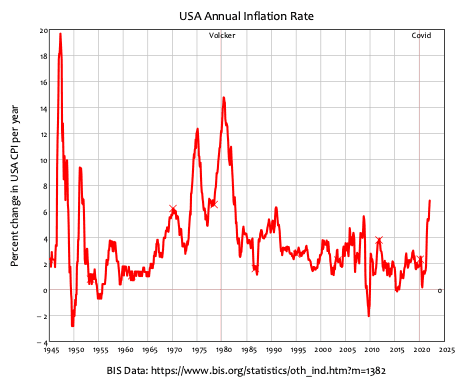
Figure 1 shows the entire history of post-World War II inflation in the USA. There were four major peaks before today’s spike, with the first two driven by Wars (the end of WWII and its price controls, and the boom in commodity prices during the Korean War). The second two, in 1975 and 1980, created modern economic theory, because they appeared to overthrow the “Keynesian” argument that fiscal policy could control both inflation and unemployment.

Figure 1: Chart showing annual change in the USA consumer price index since 1960. (Steve Keen)

“Keynesians” asserted that there was a tradeoff between inflation and unemployment: unemployment could be lowered by expansionary fiscal policy, but at the price of a higher rate of inflation. The “Keynesian” belief was that there was a negative relationship between inflation and unemployment: if inflation went up, then unemployment would go down. This was called the “Phillips Curve,” after the New Zealand engineer-turned-economist Bill Phillips, who wrote a famous empirical paper on inflation and unemployment called “The Relation between Unemployment and the Rate of Change of Money Wage Rates in the United Kingdom, 1861–1957”.

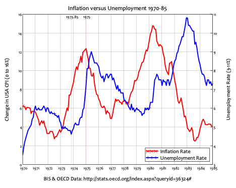
The killer blow to “Keynesian” economics was the coincidence of rising inflation and rising unemployment between late 1973 and 1975. This was dubbed stagflation, and because this was impossible according to “Keynesian” theory, Milton Friedman’s Monetarism won an intellectual battle within economics, and supplanted “Keynesianism.”

Figure 2: Chart showing rising unemployment and inflation between 1973 and 1975. (Steve Keen)

Are you sick of the inverted commas around “Keynesian” yet? Good. They’re there to make the point that this wasn’t Keynes’s theory at all, but rather how it was caricatured by the anti-Keynesian economist Milton Friedman. Trusting Friedman’s explanation of Keynesian economics is like trusting the fox’s account of why the chickens in the henhouse died.

The true inheritor of Keynes’s mantle was the renegade economist Hyman Minsky (who was the chief inspiration for my work), and he argued that credit was the main factor behind the economy’s ups and downs. When people and firms are borrowing heavily, the economy will boom, and when they borrow less or repay debt, the economy slumps. The important link, in Minsky’s genuinely Keynesian economics, is between credit and unemployment, not between inflation and unemployment.

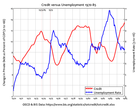
That’s obvious in the data: when credit (the annual change in private debt) is rising, unemployment falls; when credit is falling, unemployment rises. The real cause of the “stag” half of stagflation was the decline in demand as credit collapsed from 12 percent to 6 percent of GDP between September 1973 and 1976.

Figure 3: Chart showing the inverse relationship between credit (the change in private debt) and unemployment. (Steve Keen)

The “flation” bit came from two unrelated factors: the booming economy that preceded the crash of 1973, as credit doubled from 6 percent to 12 percent of GDP between 1971 and September 1973; and the Yom Kippur War, which occurred in October 1973.

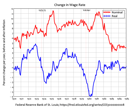
It may be hard to believe from today’s perspective, but workers had both strong trade unions and substantial bargaining power in the 1960s. Unemployment fell below 4 percent in 1966 and remained there until early 1971. It rose substantially—from 3.5 percent in 1970 to 6 percent in 1971—but fell down to a low of 4 ¾ percent in late 1973, just after the credit bubble started to burst. Workers and unions had no way of knowing in advance that this was the end of the good times—unemployment did not fall below 4 percent again until a few months in 2000, and then again before and after the COVID-19 recession—so they continued to bargain for high wage rises, which employers passed on to consumers in price rises.

Figure 4: Chart showing the annual change in nominal and inflation-adjusted wage rates. (Steve Keen)

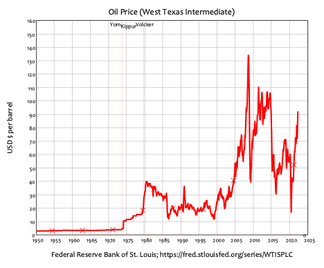
A second factor, which had never happened before, caused price rises well above the rate of wage growth: rising oil prices. Before 1973, oil prices were largely set by Big Oil: the western-owned oil companies that dominated oil drilling around the world, including in Arabian countries. They paid the oil-producing countries a pittance in royalties, and prices were low and stable—as is vividly obvious in Figure 5, where the price is a flat line between 1950 and 1973. The resentment at being paid low prices for their vital commodity motivated oil-producing countries to form OPEC (the Organization of Petroleum Exporting Countries) in 1960.

After the defeat of the Arab armies in the Yom Kippur War, OPEC launched an embargo on oil exports to the USA, which caused the oil price to increase by 250 percent, from $4.30 to $10 a barrel, in just one month.

Figure 5: Chart showing the nominal price of West Texas Crude Oil. (Steve Keen)

The coincidence of rising prices and rising unemployment therefore does have a Keynesian explanation, and the capacity for private banks to create money and additional demand by making loans plays a crucial part in it. But this wasn’t part of Friedman’s thinking at all. To him, the government was the only creator of money in the economy, and—to caricature Friedman, though more accurately than he caricatured Keynes—inflation was caused by “too much money creating too few goods.”

Friedman argued that the economy had a tendency towards what he dubbed the Non-Accelerating-Inflation-Rate-of-Unemployment—or NAIRU for short. This was set by “real” factors—people’s willingness to undergo the disutility of work, in order to receive the utility of income (in the form of either wages or profits), where this utility was measured in their physical level of consumption and not money.

A rising money supply could, however, stimulate more work, by temporarily fooling people into believing that real demand was higher than it really was: if the amount of money rose faster than the economy grew, people would initially mistake this for a higher rate of real growth in demand. Friedman then used the idea of a short-term negative relationship between unemployment and inflation to assert that this lower level of unemployment would cause a higher level of inflation.

The higher inflation would then reduce real incomes to where they were before the excessive increase in the money supply occurred. People would then come to expect this higher level of inflation to persist, while the economy settled back into its full-employment equilibrium.

Therefore, the long run effect of trying to stimulate the economy by increasing the money supply would be to increase people’s “inflationary expectations,” while leaving the level of economic activity constant at its long run equilibrium level. If the government wanted to drive the unemployment rate below the natural rate, it would have to increase the money supply even faster: hence trying to keep the unemployment rate below the natural rate required an increasing rate of growth in the money supply, and caused not merely a higher rate of inflation, but an accelerating rate of inflation. This meant that what Friedman dubbed the Long Run Phillips Curve was vertical: the relationship between unemployment and the rate of inflation was a vertical line. The only desirable point on this curve from a social welfare point of view was where inflation was zero: this was the “Non-Accelerating-Inflation-Rate-of-Unemployment.”

And speaking of inflation, this post has now exceeded my word limit! So I’ll continue it in next week’s column.